Visualizing the stock market structure

Retrieve the data from Internet

The data is from 2003 - 2008. This is reasonably calm: not too long ago so that we get high-tech firms, and before the 2008 crash. This kind of historical data can be obtained from APIs like the data.nasdaq.com and alphavantage.co.

import sys

import numpy as np
import pandas as pd

symbol_dict = {
    "TOT": "Total",
    "XOM": "Exxon",
    "CVX": "Chevron",
    "COP": "ConocoPhillips",
    "VLO": "Valero Energy",
    "MSFT": "Microsoft",
    "IBM": "IBM",
    "TWX": "Time Warner",
    "CMCSA": "Comcast",
    "CVC": "Cablevision",
    "YHOO": "Yahoo",
    "DELL": "Dell",
    "HPQ": "HP",
    "AMZN": "Amazon",
    "TM": "Toyota",
    "CAJ": "Canon",
    "SNE": "Sony",
    "F": "Ford",
    "HMC": "Honda",
    "NAV": "Navistar",
    "NOC": "Northrop Grumman",
    "BA": "Boeing",
    "KO": "Coca Cola",
    "MMM": "3M",
    "MCD": "McDonald's",
    "PEP": "Pepsi",
    "K": "Kellogg",
    "UN": "Unilever",
    "MAR": "Marriott",
    "PG": "Procter Gamble",
    "CL": "Colgate-Palmolive",
    "GE": "General Electrics",
    "WFC": "Wells Fargo",
    "JPM": "JPMorgan Chase",
    "AIG": "AIG",
    "AXP": "American express",
    "BAC": "Bank of America",
    "GS": "Goldman Sachs",
    "AAPL": "Apple",
    "SAP": "SAP",
    "CSCO": "Cisco",
    "TXN": "Texas Instruments",
    "XRX": "Xerox",
    "WMT": "Wal-Mart",
    "HD": "Home Depot",
    "GSK": "GlaxoSmithKline",
    "PFE": "Pfizer",
    "SNY": "Sanofi-Aventis",
    "NVS": "Novartis",
    "KMB": "Kimberly-Clark",
    "R": "Ryder",
    "GD": "General Dynamics",
    "RTN": "Raytheon",
    "CVS": "CVS",
    "CAT": "Caterpillar",
    "DD": "DuPont de Nemours",
}


symbols, names = np.array(sorted(symbol_dict.items())).T

quotes = []

for symbol in symbols:
    print("Fetching quote history for %r" % symbol, file=sys.stderr)
    url = (
        "https://raw.githubusercontent.com/scikit-learn/examples-data/"
        "master/financial-data/{}.csv"
    )
    quotes.append(pd.read_csv(url.format(symbol)))

close_prices = np.vstack([q["close"] for q in quotes])
open_prices = np.vstack([q["open"] for q in quotes])

# The daily variations of the quotes are what carry the most information
variation = close_prices - open_prices

Fetching quote history for np.str_('AAPL')
Fetching quote history for np.str_('AIG')
Fetching quote history for np.str_('AMZN')
Fetching quote history for np.str_('AXP')
Fetching quote history for np.str_('BA')
Fetching quote history for np.str_('BAC')
Fetching quote history for np.str_('CAJ')
Fetching quote history for np.str_('CAT')
Fetching quote history for np.str_('CL')
Fetching quote history for np.str_('CMCSA')
Fetching quote history for np.str_('COP')
Fetching quote history for np.str_('CSCO')
Fetching quote history for np.str_('CVC')
Fetching quote history for np.str_('CVS')
Fetching quote history for np.str_('CVX')
Fetching quote history for np.str_('DD')
Fetching quote history for np.str_('DELL')
Fetching quote history for np.str_('F')
Fetching quote history for np.str_('GD')
Fetching quote history for np.str_('GE')
Fetching quote history for np.str_('GS')
Fetching quote history for np.str_('GSK')
Fetching quote history for np.str_('HD')
Fetching quote history for np.str_('HMC')
Fetching quote history for np.str_('HPQ')
Fetching quote history for np.str_('IBM')
Fetching quote history for np.str_('JPM')
Fetching quote history for np.str_('K')
Fetching quote history for np.str_('KMB')
Fetching quote history for np.str_('KO')
Fetching quote history for np.str_('MAR')
Fetching quote history for np.str_('MCD')
Fetching quote history for np.str_('MMM')
Fetching quote history for np.str_('MSFT')
Fetching quote history for np.str_('NAV')
Fetching quote history for np.str_('NOC')
Fetching quote history for np.str_('NVS')
Fetching quote history for np.str_('PEP')
Fetching quote history for np.str_('PFE')
Fetching quote history for np.str_('PG')
Fetching quote history for np.str_('R')
Fetching quote history for np.str_('RTN')
Fetching quote history for np.str_('SAP')
Fetching quote history for np.str_('SNE')
Fetching quote history for np.str_('SNY')
Fetching quote history for np.str_('TM')
Fetching quote history for np.str_('TOT')
Fetching quote history for np.str_('TWX')
Fetching quote history for np.str_('TXN')
Fetching quote history for np.str_('UN')
Fetching quote history for np.str_('VLO')
Fetching quote history for np.str_('WFC')
Fetching quote history for np.str_('WMT')
Fetching quote history for np.str_('XOM')
Fetching quote history for np.str_('XRX')
Fetching quote history for np.str_('YHOO')

Learning a graph structure

We use sparse inverse covariance estimation to find which quotes are correlated conditionally on the others. Specifically, sparse inverse covariance gives us a graph, that is a list of connections. For each symbol, the symbols that it is connected to are those useful to explain its fluctuations.

from sklearn import covariance

alphas = np.logspace(-1.5, 1, num=10)
edge_model = covariance.GraphicalLassoCV(alphas=alphas)

# standardize the time series: using correlations rather than covariance
# former is more efficient for structure recovery
X = variation.copy().T
X /= X.std(axis=0)
edge_model.fit(X)

GraphicalLassoCV(alphas=array([ 0.03162278,  0.05994843,  0.11364637,  0.21544347,  0.40842387,
        0.77426368,  1.46779927,  2.7825594 ,  5.27499706, 10.        ]))

Clustering using affinity propagation

We use clustering to group together quotes that behave similarly. Here, amongst the various clustering techniques available in the scikit-learn, we use Affinity Propagation as it does not enforce equal-size clusters, and it can choose automatically the number of clusters from the data.

Note that this gives us a different indication than the graph, as the graph reflects conditional relations between variables, while the clustering reflects marginal properties: variables clustered together can be considered as having a similar impact at the level of the full stock market.

from sklearn import cluster

_, labels = cluster.affinity_propagation(edge_model.covariance_, random_state=0)
n_labels = labels.max()

for i in range(n_labels + 1):
    print(f"Cluster {i + 1}: {', '.join(names[labels == i])}")

Cluster 1: Apple, Amazon, Yahoo
Cluster 2: Comcast, Cablevision, Time Warner
Cluster 3: ConocoPhillips, Chevron, Total, Valero Energy, Exxon
Cluster 4: Cisco, Dell, HP, IBM, Microsoft, SAP, Texas Instruments
Cluster 5: Boeing, General Dynamics, Northrop Grumman, Raytheon
Cluster 6: AIG, American express, Bank of America, Caterpillar, CVS, DuPont de Nemours, Ford, General Electrics, Goldman Sachs, Home Depot, JPMorgan Chase, Marriott, McDonald's, 3M, Ryder, Wells Fargo, Wal-Mart
Cluster 7: GlaxoSmithKline, Novartis, Pfizer, Sanofi-Aventis, Unilever
Cluster 8: Kellogg, Coca Cola, Pepsi
Cluster 9: Colgate-Palmolive, Kimberly-Clark, Procter Gamble
Cluster 10: Canon, Honda, Navistar, Sony, Toyota, Xerox

Embedding in 2D space

For visualization purposes, we need to lay out the different symbols on a 2D canvas. For this, we use Manifold learning techniques to retrieve 2D embedding. We use a dense eigen_solver to achieve reproducibility (arpack is initiated with the random vectors that we do not control). In addition, we use a large number of neighbors to capture the large-scale structure.

# Finding a low-dimension embedding for visualization: find the best position of
# the nodes (the stocks) on a 2D plane

from sklearn import manifold

node_position_model = manifold.LocallyLinearEmbedding(
    n_components=2, eigen_solver="dense", n_neighbors=6
)

embedding = node_position_model.fit_transform(X.T).T

Visualization

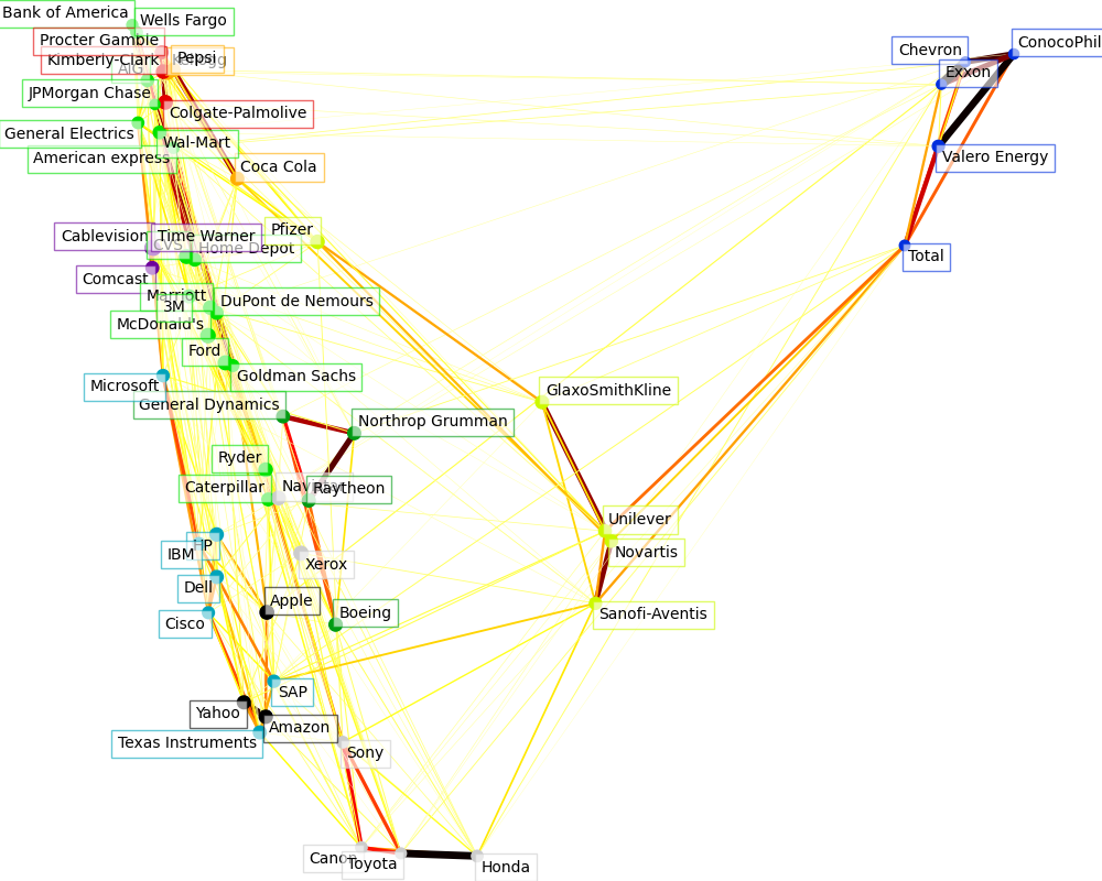
The output of the 3 models are combined in a 2D graph where nodes represent the stocks and edges the connections (partial correlations):

• cluster labels are used to define the color of the nodes
• the sparse covariance model is used to display the strength of the edges
• the 2D embedding is used to position the nodes in the plan

This example has a fair amount of visualization-related code, as visualization is crucial here to display the graph. One of the challenges is to position the labels minimizing overlap. For this, we use an heuristic based on the direction of the nearest neighbor along each axis.

import matplotlib.pyplot as plt
from matplotlib.collections import LineCollection

plt.figure(1, facecolor="w", figsize=(10, 8))
plt.clf()
ax = plt.axes([0.0, 0.0, 1.0, 1.0])
plt.axis("off")

# Plot the graph of partial correlations
partial_correlations = edge_model.precision_.copy()
d = 1 / np.sqrt(np.diag(partial_correlations))
partial_correlations *= d
partial_correlations *= d[:, np.newaxis]
non_zero = np.abs(np.triu(partial_correlations, k=1)) > 0.02

# Plot the nodes using the coordinates of our embedding
plt.scatter(
    embedding[0], embedding[1], s=100 * d**2, c=labels, cmap=plt.cm.nipy_spectral
)

# Plot the edges
start_idx, end_idx = non_zero.nonzero()
# a sequence of (*line0*, *line1*, *line2*), where::
#            linen = (x0, y0), (x1, y1), ... (xm, ym)
segments = [
    [embedding[:, start], embedding[:, stop]] for start, stop in zip(start_idx, end_idx)
]
values = np.abs(partial_correlations[non_zero])
lc = LineCollection(
    segments, zorder=0, cmap=plt.cm.hot_r, norm=plt.Normalize(0, 0.7 * values.max())
)
lc.set_array(values)
lc.set_linewidths(15 * values)
ax.add_collection(lc)

# Add a label to each node. The challenge here is that we want to
# position the labels to avoid overlap with other labels
for index, (name, label, (x, y)) in enumerate(zip(names, labels, embedding.T)):
    dx = x - embedding[0]
    dx[index] = 1
    dy = y - embedding[1]
    dy[index] = 1
    this_dx = dx[np.argmin(np.abs(dy))]
    this_dy = dy[np.argmin(np.abs(dx))]
    if this_dx > 0:
        horizontalalignment = "left"
        x = x + 0.002
    else:
        horizontalalignment = "right"
        x = x - 0.002
    if this_dy > 0:
        verticalalignment = "bottom"
        y = y + 0.002
    else:
        verticalalignment = "top"
        y = y - 0.002
    plt.text(
        x,
        y,
        name,
        size=10,
        horizontalalignment=horizontalalignment,
        verticalalignment=verticalalignment,
        bbox=dict(
            facecolor="w",
            edgecolor=plt.cm.nipy_spectral(label / float(n_labels)),
            alpha=0.6,
        ),
    )

plt.xlim(
    embedding[0].min() - 0.15 * np.ptp(embedding[0]),
    embedding[0].max() + 0.10 * np.ptp(embedding[0]),
)
plt.ylim(
    embedding[1].min() - 0.03 * np.ptp(embedding[1]),
    embedding[1].max() + 0.03 * np.ptp(embedding[1]),
)

plt.show()

Total running time of the script: (0 minutes 2.861 seconds)

Download Jupyter notebook: plot_stock_market.ipynb

Download Python source code: plot_stock_market.py

Download zipped: plot_stock_market.zip

Related examples

Manifold learning on handwritten digits: Locally Linear Embedding, Isomap…

Comparison of Manifold Learning methods

Various Agglomerative Clustering on a 2D embedding of digits

Segmenting the picture of greek coins in regions